The fitted curves give the trapped charge per pixel in ADU after illumination at the given level for any given time. To make it simpler to characterise the data, single exponentials have been used that fit the data fairly well. The following important points can be deduced:
- RBI effects are seen at all levels of illumination; the strength of the RBI effect seems to be independent of saturation of the CCD chip, and saturation is not a necessary condition for it to occur.
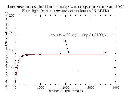
- For long exposures at low levels of illumination, the CCD can be saturated whilst the equilibrium number of filled traps is small. A saturated CCD does not necessarily mean a large RBI effect.
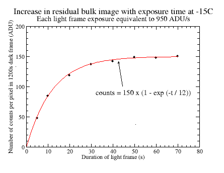
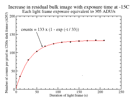
- The time-constant for charging the traps depends on the incident flux; a higher intensity of illumination gives a shorter time-constant.
- The number of filled traps for a given intensity appears to reach a dynamic equilibrium when the number of decays per unit time equals the number of traps being filled. This steady-state number of filled traps depends on the incident flux; a higher intensity of illumination gives a higher number of filled traps.
- There is a maximum number of traps per pixel which is not exceeded even for long periods of intense illumination. For this chip, the number of filled traps is equivalent to about 180 ADU or 240 electrons per pixel.
A simple model for RBI
The main features of the RBI behaviour can be explained with a simple model as follows. Suppose that the rate at which the traps are charged is proportional to the number of unfilled traps (i.e. when all traps are empty, any photo-electron in the substrate finds a trap and so they initially fill quickly; when most are full, the chances are that an electron won't encounter an unfilled trap so the rate of charging is slower). Further suppose that the rate of decrease of the number of filled traps is proportional to the number of traps that are currently filled (i.e. assume that the traps decay at random; the more traps that are filled, the more decays there will be in any given time). Here for the sake of simplicity we are assuming just one decay time-constant, although the analysis above shows there to be at least two.
Expressing this mathematically, we have:
which has the solution:
where:
- n is the number of filled traps at time t
- N is the total number of traps
- I is the number of photo-electrons generated per second
- k1 x N is the probability of a photo-electron being generated in the substrate
- k2 is the probability of trap decay per second
From this equation, we see that the time-constant for charging the traps is given by:

and the ultimate steady-state number of charged traps is:
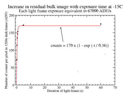
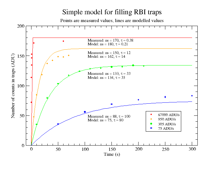
From the analysis above, the measured decay time-constants are 135s and 455s. If we choose the smaller of the two time constants as being dominant, then k2 = 1/135. After a bit of experimentation, a suitable value for k1 of 0.00007 is found. Using the four values for I from above (i.e. 67000 ADU/s, 950 ADU/s, 305 ADU/s and 75 ADU/s), the estimated number of counts in the traps can be calculated at any time t. A value of 180 ADU for the maximum number of filled traps per pixel has been adopted and the results are shown in the graph below.
Thermal dependency of RBI: trap decay
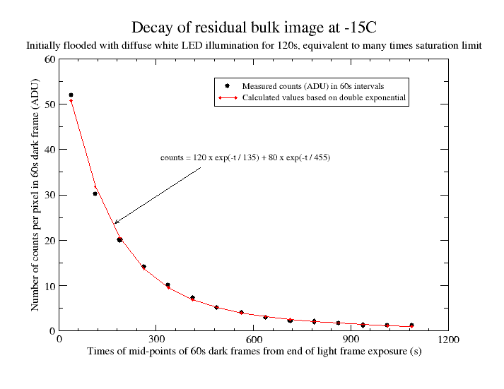
To assess the thermal dependence of the RBI effect, the rate of decay was measured at various temperatures using the same procedure as above. The results are shown below.
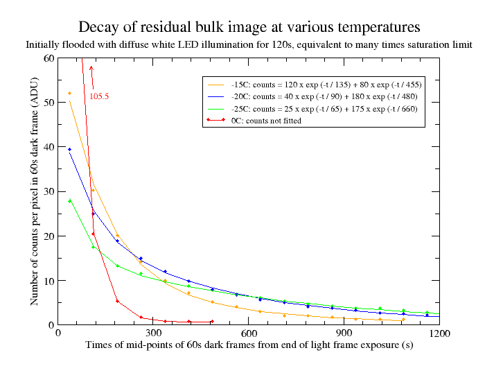
The orange points plot the same data at -15C as the graph at the top of the page. The blue and green points are for -20C and -25C. The fitted curves show that the longer time-constant increases and becomes more dominant at lower temperatures. (The apparent reduction in the shorter time-constant may be just an artifact of the double-exponential fit). In terms of the simple model above, we can say that the probability of trap decay per second, k2, decreases with decreasing temperature.
The red points show the trap decay at 0C. Note how this is very much more rapid; after about five minutes there is little residual image at all. This suggests an alternative method for managing RBI for this chip: image framing and focussing could be done at warmer temperatures where trap decay is rapid, and then the CCD could be cooled to its imaging temperature. (But note that it is not necessarily desirable to start with empty traps when making photometric measurements; see below).
In practice for this camera, a delay of five minutes after focussing at 0C allows all the traps to empty and about another five minutes would elapse before the camera stabilised at a lower target temperature. That implies a ten-minute wait, after which time any RBI effect would in any case be small even if the camera had been held at a constant temperature of -25C. However, for other chips where the RBI effect is much greater, image framing and focussing before cooling the chip may be worth considering.
(The standard method for managing RBI is to pre-flash the CCD with near-IR illumination to fill all the traps before an exposure. But the CCD must be cooled quite substantially to decrease the decay time-constant to the point where trap decay does not significantly increase the noise in the exposure, and this is not always achievable).
Thermal dependency of RBI: trap charging
Trap charging was measured in the same way as before, except a dark frame of 2700 seconds duration was taken following each light frame exposure in order to capture all the trap decay at -25C. The white LED light source was used, and in addition exposures were also made with illumination by miniature incandescent bulbs. The same light box was used in both cases; the source is switchable between LED and incandescent.
The LED measurements were made after covering an extension tube screwed to the front of the camera with 16 thicknesses of printer paper. Such is the sensitivity of the camera in the infra-red that 48 thicknesses of printer paper were required(!) for the incandescent illumination and the camera had to be moved twice as far from the light box, even though the LED and incandescent output look about the same by eye. The incident flux was adjusted to match the value of 305 ADU/s used at -15C as closely as possible and the results are shown below.

The orange points are for the incandescent illumination and the green points are for white LEDs. The red line is a mean fit to both sets of data. The blue points are for the measurements made at -15C given above and are for comparison purposes. For all curves, the average illumination over the course of the measurements is given.
Note the following points about these curves:
- The equilibrium number of filled traps for a given incident flux is higher at lower temperatures, because the traps decay at a slower rate. If we assume in the simple model that k1 is unchanged with temperature and adopt a value for k2 of 1/660 (based on the decay measurements at -25C) then the expected equilibrium number of traps is equivalent to 168 ADU - a bit higher than the measured value of 154 ADU. The expected time-constant is about 44 seconds which is rather longer than the measured 34 seconds; surprisingly the measured value does not seem to have changed very much with temperature.
- The curve obtained for incandescent illumination is almost the same as that for white LED illumination. This is a rather unsophisticated measurement; it is assumed that the incandescent illumination resulted in a higher infrared flux, although re-emission of visible photons from the white LED illumination as infrared (after absorption in the paper used to adjust the level of illumination) could have made a contribution. According to the simple model, a 25% increase in k1 (i.e. an increase in the probability of photo-electron generation in the substrate) would decrease the time-constant by about 20%. Since the measured time-constants for the LED and incandescent illumination are the same, it seems that the value of k1 does not vary significantly over the tested wavelength range.
Consequences of RBI effects for photometry
Consider a single CCD well and define Nw as the number of electrons that would be in that well if none were trapped in the substrate and Nt as the number of trapped electrons. Then we define the percent absolute photometric error as:
The theoretical value of Nw is equal to I x t and increases linearly with time depending on the incident flux. Nt varies as shown in the graphs above. The following graph shows how the percent absolute photometric error varies with the number of counts per pixel. The two curves are for incident fluxes equivalent to 305 ADU/s and 75 ADU/s, based on the measured values for Nt at -15C and assuming that all the traps are initially empty. (Of course the true situation is a bit more complicated than this; a photometric measurement of a star comprises a number of pixels of different numbers of counts).
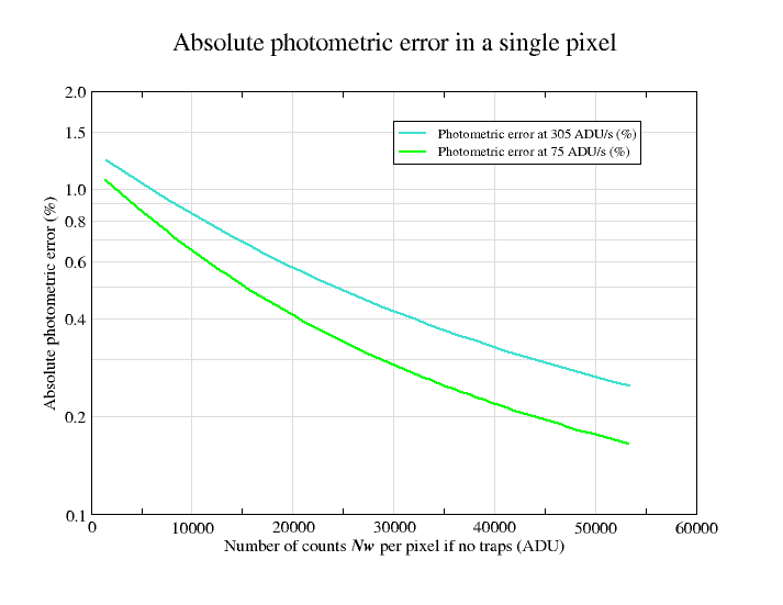
We can see from the graph that RBI effects have the greatest influence when the total number of counts is small, for any given incident flux. (In fact it can be shown, for the simple model at least, that the maximum expected photometric error is equal to the probability of a photo-electron being generated in the substrate, assuming that all such electrons are initially trapped when all the traps are empty. From above, we see that this probability is given by k1 x N, which equals 0.013 for the chosen value of k1, or 1.3%). However, assuming that a typical photometric measurement contains sufficient counts to give a good signal to noise ratio, the influences of RBI effects for this chip are likely to be very small, even for absolute photometric measurements. Note that a photometric error of 0.5% is equivalent to only 5 millimagnitude.
Many photometric measurements are not absolute measurements but are obtained by taking the ratio of counts in different wells for the object of interest and a comparison object. For stellar photometry, it is sensible to follow the general advice that stars of similar brightness and colour should be compared; this helps to ensure that the target and comparison object are affected in a similar way. In this case, the RBI effect on the true ratio can probably be reduced to one or two millimagnitude.
If the traps are already charged to their equilibrium values prior to the start of the exposure, then the consequences of the RBI effect can in principle be reduced to zero. In this case, the rate of trap decay during the exposure equals the rate of charging and there is no net effect on the measured counts in the CCD wells. There will always be some variation in count rate across adjacent pixels due to imperfect telescope tracking and atmospheric scintillation so exact equilibrium is unlikely to be achieved in practice. This might be mitigated to some extent by oversampling the target (i.e. spreading the light across more pixels) to reduce the pixel-to-pixel variation. For highest accuracy time-series photometry taken during a single night (e.g. for expolanet transits), it may be sensible to make exposures continuously, in order to keep the traps charged to near their equilibrium values.
Note that whilst the RBI effects are small, they are not negligible for all circumstances. It is advisable not to follow flat field exposures immediately with dark or bias frames, for example. However, a little thought given to planning the sequence of exposures during the course of a night can readily mitigate the effects of RBI with this chip, and the use of infra-red pre-flash seems like an unnecessary complication.