Periodic Error Correction for Losmandy Gemini
What is periodic error and why is it a problem?
Periodic error is a repetitive variation in the tracking rate of a motor-driven telescope mount. It can result in blurred long-exposure images, where each star appears to be sretched into an oval shape. The size of the effect depends on the size of the error and the image scale: images taken with short focal length telescopes on good quality mounts may not show periodic error effects at all. But in many imaging situations with typical amateur telescope mounts, periodic error is a nuisance that has to be compensated for in some way.
What causes periodic error?
Periodic error is generally caused by imperfect gears or mis-aligned bearings. Many telescope drives in the amateur market typically use a motor driving a worm gear via a gear box. The worm gear meshes with a spur gear that is directly attached to the right ascension axis of the mount. The worm gear typically rotates once in a few minutes and causes the spur gear to advance by one tooth as it does so. Ideally, the worm gear would have a perfectly smooth and uniform spiral surface and the spur gear and gearbox gears would have perfectly cut teeth. Manufacturing tolerances mean that this is not achieved in practice so the worm does not cause completely uniform rotation of the spur gear. This non-uniform motion repeats for each period of rotation of the worm gear and is usually the largest source of periodic error. (Note that there are some other designs available that use direct-drive motors, belt drives or friction drives. These may show little or no error, or the error that does occur may be non-periodic).
Periodic error correction
Most modern telescope controllers allow the user to program a periodic error correction so that the rate of rotation of the worm gear is modified by the controller. This can reduce the periodic error and may mean that fewer autoguiding corrections are required. Periodic error corrections are usually calculated by determining a star's apparent drift over a number of worm cycles and then taking an average. It is unlikely that periodic error will be removed completely, since the actual drift tends to vary from one cycle to the next due to irregularities in the spur gear teeth.
The following sections describe the operation of a straightforward program that will analyse star position data and calculate the necessary corrections for a Losmandy Gemini unit (this has been tested using Gemini I, but not yet with Gemini II). The program is a Scilab script. You will need to download version 6.0 or higher of Scilab from www.scilab.org if you don't already have it, or there may be a package for your Linux distribution.
Getting star position data with GoQat
You can get the necessary data using GoQat with an autoguider camera. On the Autoguider tab, click the 'Advanced...' button and choose the options to write the star position and worm position data. After logging the star position for a number of worm periods, edit the "star_pos.csv" file in the GoQat folder of your home directory and select the rows that you want, then paste directly into a new text file and save the file. The first column is time in seconds, the second column is the worm position, the next column is the declination position of the star and the last column is the right ascension position. The Scilab script does not require the second column to be present but you will need to provide a column of worm position data if you want to create a PEC file.
Note that if GoQat loses the star when recording the data, it will write "Nan" (Not a number) to "star_pos.csv". You will need to find and remove any Nan's before Scilab will read the file successfully.
Running the GeminiPEC script
Before you run the script, you might wish to customise some of the default values. To do that, load the script into your favourite editor and find the section near the top marked "// SET DEFAULT VALUES HERE". You can also override these values when you run the script.
Start Scilab and load the script with the command:
exec('/PATH/GeminiPEC.sce');
where "/PATH/" is the location where you have installed the script. Note the trailing ";" to stop Scilab listing the enire script to the command window.
When the script has loaded, you will see the following dialog box:

|
Click the "Choose input file..." button and choose your edited file of star position data. A window is displayed showing the right ascension and declination positions of the star plotted against time. Select the region of data that you want to analyse by entering values in the "Start time (s)" and "Num. worm periods" fields in the dialog box. The script fills these values in for you depending on the data in the file but you can change them if you wish. Note that the minimum number of worm periods must be at least three. The other dialog box fields are filled according to the defaults in the GeminiPEC script; you can override them here if you want. The fields are as follows:
The other items are described below. |
When you have selected the desired data range for analysis, click "Run". There may be a pause whilst Scilab analyses the data. When the calculations are done, the following three windows are displayed:
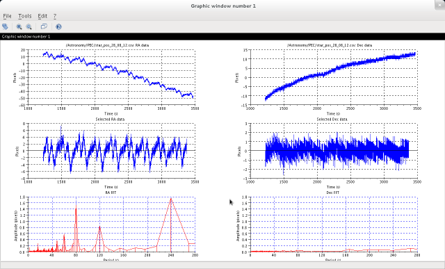
First window:
- The top two graphs show the raw right ascension and declination position of the star against time, with the vertical axis in camera pixels.
- The next two graphs show the selected portion of the data optionally de-rotated by the chosen camera angle (see below) and with any long-term trend removed.
- The bottom pair of graphs show the fourier analysis of the selected data, plotting the amplitude in arcsec of each component against its period, using the pixel to arcsec conversion factors entered in the "RA arcsec/pixel" and "Dec arcsec/pixel" fields of the initial dialog box. The three main peaks contribute periods of 80s, 120s and 240s to the right ascension data (reading from left to right) in this example.
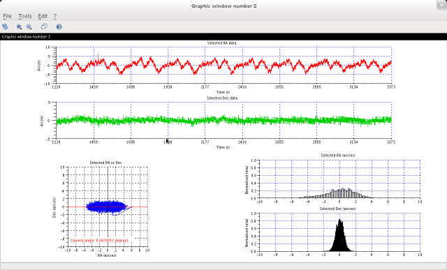
Second window:
- The top two graphs show the variation in right ascension and declination position of the star against time with any long-term trend removed in the selected data. In this example, an Ovision worm and Mclennan gear box were used and the maximum amplitude of the error lies within the 5 arcsec Ovision guarantee.
- The bottom left-hand graph plots the measured declination position against the measured right ascension position (after removal of long-term drift). This elongated blob gives some idea of the expected shape of a star on a long-exposure image resulting from periodic error alone. (Actually this exaggerates the effect because the central areas, where the star spends more time, would be brighter in practice). The orientation of the camera can be estimated from the shape of this plot. For example, if the plot is stretched along a line sloping at 45 degrees from bottom left to top right, then the camera must have been rotated at -45 degrees relative to the east-west axis. You should adjust this by entering 45 degrees in the "Camera angle (deg)" field of the initial dialog box to correct the net rotation to zero. Click "Run" again to re-calculate.
- The bottom right-hand pair of graphs show histograms of the star's right ascension and declination positions after removal of long-term drift. The declination positon shows a good gaussian distribution as might be expected from seeing effects alone, whereas the right acension histogram is smeared by periodic error.
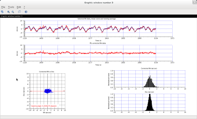
Third window:
- The top graph shows the actual range of data that has been used to calculate an average star postion curve. For computational reasons, this is always one worm cycle fewer than the number selected originally. The red curve is the star's measured right ascension position plotted against time, with any long-term trend removed. The blue curve is the average of all selected worm cycles and repeats exactly from one worm period to the next. The black curve is a smoothed version of the blue curve, using a running average specified in the "Running avg. (s)" field of the initial dialog box. It is this smoothed version of the star's position, averaged over a number of worm cycles, that is used to generate the periodic error correction data.
- The second graph shows what would happen if the black curve were to be subtracted from the red curve - in other words it is the residual right ascension motion of the star if the periodic error was exactly corrected. This is the absolute best that you could expect to see. In practice, the correction is never this good and there is always some residual periodic error.
- The bottom left-hand graph plots the measured declination position against the residual right ascension position from the second graph. This gives some idea of the expected shape of a star on a long-exposure image after perfect periodic error correction. It will not be this good in reality.
- The bottom right-hand pair of graphs show histograms of the star's residual right ascension position and measured declination positions. The right acension histogram is now much tighter compared with the same graph in the second graphics window, but the remaining periodic error that always occurs in practice will make it worse than this.
Generating periodic error correction data
If your input file contains worm postion data, you can generate a periodic error correction file for loading into a Losmandy Gemini controller with GoQat. You will need to set the following values in the initial dialog box:
- Guide speed - It is strongly recommended that you choose the lowest possible value for the "Guide speed" parameter. For the Gemini I controller, this is 0.2 times sidereal rate. This permits more corrections to be made per worm cycle and gives a smoother result. If you load the PEC corrections file via GoQat, GoQat will set your controller to this selected speed automatically. Any autoguiding corrections that you may make must also be done at this speed. But a value of 0.2 should be ideal for all but the most wildly erratic mounts.
- RA drift correction - You can attempt to correct any long-term drift in right ascension, such as shown in the first graphics window, by clicking the "Correct RA drift?" checkbox.
- PEC shift - If you restart the Gemini I controller after a battery change or do a cold restart it will reset the assumed current worm position to zero. This will invalidate any worm position data that you recorded with your star position data. However, GoQat stores the final worm position if you instruct GoQat to park the telescope and you can enter this value in the "PEC shift (steps)" field to recalculate the PEC corrections using your previous star and worm position data. You can also enter a value in this field if you want the PEC corrections to be replayed slightly sooner in anticipation of any upcoming error. For example, if the encoder has 6400 steps per revolution and one revolution takes 240 seconds, then a value of 13 will cause the PEC correction to occur about half a second early (13/6400 * 240 = 0.5).
- Invert PEC - If the periodic error is much worse after applying the correction, then click the "Invert PEC?" checkbox.
To generate the PEC data, click the "Write data files?" checkbox and then click "Run". Scilab writes the following data files in the same location as the input data file, where FILENAME is the name of your input data file:
- FILENAME.fft - Contains the fourier transform data. The first column is the period in seconds, the second column is the amplitude of any component in the right ascension data with that period and the third column is the amplitude of any component in the declination data with that period. The amplitudes are in arcsec.
- FILENAME.RaDec - Contains the right ascension and declination variation in arcsec for the selected data, optionally de-rotated by the value in the "Camera angle (deg)" field, with any long-term trend removed. The first column is the time in seconds, the second column is the right acension data and the third column is the declination data.
- FILENAME.wp_Ra - Contains one worm cycle of right ascension star position data, in arcsec. The right ascension data is the mean over the number of worm cycles selected for analysis and is smoothed by the specified running average. The first column is the worm position and the second column is the right ascension data.
- FILENAME.PEC - Contains the east and west corrections and durations for loading into the Gemini controller to correct the periodic error. The first column is the guide correction direction (east or west), the second column is the worm position at which to apply this correction and the third column is the number of steps to apply the correction. There are two header records; the first is the number of encoder steps for one worm rotation and the second is the guide speed for which the corrections have been calculated. GoQat uses these values when loading the data into the Gemini controller. If you aren't using GoQat, then remove these first two records and load the file into the controller by some other method.
When you have created the PEC file, you can load it into the Gemini controller using GoQat. The GoQat manual tells you how to do this. Remember to turn PEC on after loading the data.
Please note that there are other more sophisticated programs available for periodic error analysis that calculate the necessary corrections for various drive controllers.
An example of periodic error correction
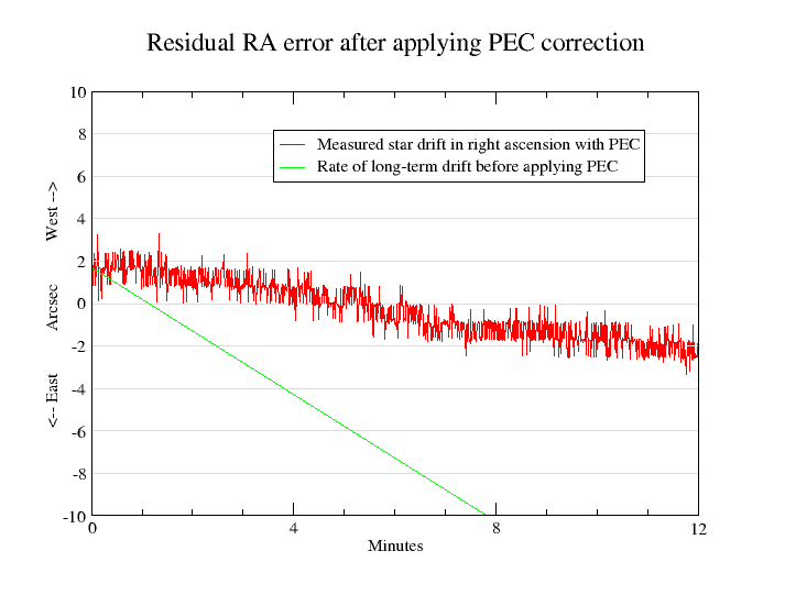
The following graph shows an example of residual error after applying PEC. There is still some long-term drift, probably due to polar misalignment. Some attempts are more successful than others because periodic error seems to vary with mount loading, pointing direction and maybe temperature as the gears engage slightly differently. (Of course it would be possible to generate a number of PEC correction files for different conditions and use them as appropriate). Nonetheless, in the best cases the error is very much reduced. The sudden changes in speed that make guiding so hard have been eliminated - see the top graph of the third graphics window above for comparison.